MATLAB compatibility module¶

This module contains a number of functions that emulate some of the functionality of MATLAB. The intent of these functions is to provide a simple interface to the python control systems library (python-control) for people who are familiar with the MATLAB Control Systems Toolbox (tm). Most of the functions are just calls to python-control functions defined elsewhere. To include all of the functions described here, use:

from control.matlab import *

The following tables give an overview of the module control.matlab. They also show the implementation progress and the planned features of the module.

The symbols in the first column show the current state of a feature:

* : The feature is currently implemented.
- : The feature is not planned for implementation.
s : A similar feature from another library (Scipy) is imported into the module, until the feature is implemented here.

Creating linear models¶

*	`tf()`	create transfer function (TF) models
	zpk	create zero/pole/gain (ZPK) models.
*	`ss()`	create state-space (SS) models
	dss	create descriptor state-space models
	delayss	create state-space models with delayed terms
*	`frd()`	create frequency response data (FRD) models
	lti/exp	create pure continuous-time delays (TF and ZPK only)
	filt	specify digital filters
-	lti/set	set/modify properties of LTI models
-	setdelaymodel	specify internal delay model (state space only)
*	`rss()`	create a random continuous state space model
*	`drss()`	create a random discrete state space model

Data extraction¶

*	`tfdata()`	extract numerators and denominators
	lti/zpkdata	extract zero/pole/gain data
	lti/ssdata	extract state-space matrices
	lti/dssdata	descriptor version of SSDATA
	frd/frdata	extract frequency response data
	lti/get	access values of LTI model properties
	ss/getDelayModel	access internal delay model (state space)

Conversions¶

*	`tf()`	conversion to transfer function
	zpk	conversion to zero/pole/gain
*	`ss()`	conversion to state space
*	`frd()`	conversion to frequency data
*	`c2d()`	continuous to discrete conversion
	d2c	discrete to continuous conversion
	d2d	resample discrete-time model
	upsample	upsample discrete-time LTI systems
*	`ss2tf()`	state space to transfer function
s	`ss2zpk()`	transfer function to zero-pole-gain
*	`tf2ss()`	transfer function to state space
s	`tf2zpk()`	transfer function to zero-pole-gain
s	`zpk2ss()`	zero-pole-gain to state space
s	`zpk2tf()`	zero-pole-gain to transfer function

System interconnections¶

*	`append()`	group LTI models by appending inputs/outputs
*	`parallel()`	connect LTI models in parallel (see also overloaded `+`)
*	`series()`	connect LTI models in series (see also overloaded `*`)
*	`feedback()`	connect lti models with a feedback loop
	lti/lft	generalized feedback interconnection
*	`connect()`	arbitrary interconnection of lti models
	sumblk	summing junction (for use with connect)
	strseq	builds sequence of indexed strings (for I/O naming)

System gain and dynamics¶

*	`dcgain()`	steady-state (D.C.) gain
	lti/bandwidth	system bandwidth
	lti/norm	h2 and Hinfinity norms of LTI models
*	`pole()`	system poles
*	`zero()`	system (transmission) zeros
	lti/order	model order (number of states)
*	`pzmap()`	pole-zero map (TF only)
	lti/iopzmap	input/output pole-zero map
*	`damp()`	natural frequency, damping of system poles
	esort	sort continuous poles by real part
	dsort	sort discrete poles by magnitude
	lti/stabsep	stable/unstable decomposition
	lti/modsep	region-based modal decomposition

Time-domain analysis¶

*	`step()`	step response
	stepinfo	step response characteristics
*	`impulse()`	impulse response
*	`initial()`	free response with initial conditions
*	`lsim()`	response to user-defined input signal
	lsiminfo	linear response characteristics
	gensig	generate input signal for LSIM
	covar	covariance of response to white noise

Frequency-domain analysis¶

*	`bode()`	Bode plot of the frequency response
	lti/bodemag	Bode magnitude diagram only
	sigma	singular value frequency plot
*	`nyquist()`	Nyquist plot
*	`nichols()`	Nichols plot
*	`margin()`	gain and phase margins
	lti/allmargin	all crossover frequencies and margins
*	`freqresp()`	frequency response over a frequency grid
*	`evalfr()`	frequency response at single frequency

Model simplification¶

*	`minreal()`	minimal realization; pole/zero cancellation
	ss/sminreal	structurally minimal realization
*	`hsvd()`	hankel singular values (state contributions)
*	`balred()`	reduced-order approximations of LTI models
*	`modred()`	model order reduction

Compensator design¶

*	`rlocus()`	evans root locus
*	`place()`	pole placement
	estim	form estimator given estimator gain
	reg	form regulator given state-feedback and estimator gains

LQR/LQG design¶

	ss/lqg	single-step LQG design
*	`lqr()`	linear quadratic (LQ) state-fbk regulator
	dlqr	discrete-time LQ state-feedback regulator
	lqry	LQ regulator with output weighting
	lqrd	discrete LQ regulator for continuous plant
	ss/lqi	Linear-Quadratic-Integral (LQI) controller
	ss/kalman	Kalman state estimator
	ss/kalmd	discrete Kalman estimator for cts plant
	ss/lqgreg	build LQG regulator from LQ gain and Kalman estimator
	ss/lqgtrack	build LQG servo-controller
	augstate	augment output by appending states

State-space (SS) models¶

*	`rss()`	random stable cts-time state-space models
*	`drss()`	random stable disc-time state-space models
	ss2ss	state coordinate transformation
	canon	canonical forms of state-space models
*	`ctrb()`	controllability matrix
*	`obsv()`	observability matrix
*	`gram()`	controllability and observability gramians
	ss/prescale	optimal scaling of state-space models.
	balreal	gramian-based input/output balancing
	ss/xperm	reorder states.

Frequency response data (FRD) models¶

	frd/chgunits	change frequency vector units
	frd/fcat	merge frequency responses
	frd/fselect	select frequency range or subgrid
	frd/fnorm	peak gain as a function of frequency
	frd/abs	entrywise magnitude of frequency response
	frd/real	real part of the frequency response
	frd/imag	imaginary part of the frequency response
	frd/interp	interpolate frequency response data
*	`mag2db()`	convert magnitude to decibels (dB)
*	`db2mag()`	convert decibels (dB) to magnitude

Time delays¶

	lti/hasdelay	true for models with time delays
	lti/totaldelay	total delay between each input/output pair
	lti/delay2z	replace delays by poles at z=0 or FRD phase shift
*	`pade()`	pade approximation of time delays

Model dimensions and characteristics¶

	class	model type (‘tf’, ‘zpk’, ‘ss’, or ‘frd’)
	isa	test if model is of given type
	tf/size	model sizes
	lti/ndims	number of dimensions
	lti/isempty	true for empty models
	lti/isct	true for continuous-time models
	lti/isdt	true for discrete-time models
	lti/isproper	true for proper models
	lti/issiso	true for single-input/single-output models
	lti/isstable	true for models with stable dynamics
	lti/reshape	reshape array of linear models

Overloaded arithmetic operations¶

*	+ and -	add, subtract systems (parallel connection)
*	*	multiply systems (series connection)
	/	right divide – sys1*inv(sys2)
-	\	left divide – inv(sys1)*sys2
	^	powers of a given system
	‘	pertransposition
	.’	transposition of input/output map
	.*	element-by-element multiplication
	[..]	concatenate models along inputs or outputs
	lti/stack	stack models/arrays along some dimension
	lti/inv	inverse of an LTI system
	lti/conj	complex conjugation of model coefficients

Matrix equation solvers and linear algebra¶

*	`lyap()`	solve continuous-time Lyapunov equations
*	`dlyap()`	solve discrete-time Lyapunov equations
	lyapchol, dlyapchol	square-root Lyapunov solvers
*	`care()`	solve continuous-time algebraic Riccati equations
*	`dare()`	solve disc-time algebraic Riccati equations
	gcare, gdare	generalized Riccati solvers
	bdschur	block diagonalization of a square matrix

Additional functions¶

*	`gangof4()`	generate the Gang of 4 sensitivity plots
*	`linspace()`	generate a set of numbers that are linearly spaced
*	`logspace()`	generate a set of numbers that are logarithmically spaced
*	`unwrap()`	unwrap phase angle to give continuous curve

control.matlab.bode(*args, **keywords)¶

Bode plot of the frequency response

Plots a bode gain and phase diagram

Parameters:

sys : LTI, or list of LTI

System for which the Bode response is plotted and give. Optionally a list of systems can be entered, or several systems can be specified (i.e. several parameters). The sys arguments may also be interspersed with format strings. A frequency argument (array_like) may also be added, some examples: * >>> bode(sys, w) # one system, freq vector * >>> bode(sys1, sys2, ..., sysN) # several systems * >>> bode(sys1, sys2, ..., sysN, w) * >>> bode(sys1, ‘plotstyle1’, ..., sysN, ‘plotstyleN’) # + plot formats

omega: freq_range

Range of frequencies in rad/s

dB : boolean

If True, plot result in dB

Hz : boolean

If True, plot frequency in Hz (omega must be provided in rad/sec)

deg : boolean

If True, return phase in degrees (else radians)

Plot : boolean

If True, plot magnitude and phase

Examples

>>> sys = ss("1. -2; 3. -4", "5.; 7", "6. 8", "9.")
>>> mag, phase, omega = bode(sys)

Todo

Document these use cases

```
>>> bode(sys, w)
```
```
>>> bode(sys1, sys2, ..., sysN)
```
```
>>> bode(sys1, sys2, ..., sysN, w)
```

>>> bode(sys1, 'plotstyle1', ..., sysN, 'plotstyleN')

control.matlab.c2d(sysc, Ts, method='zoh')¶

Return a discrete-time system

Parameters:

sysc: LTI (StateSpace or TransferFunction), continuous

System to be converted

Ts: number

Sample time for the conversion

method: string, optional

Method to be applied, ‘zoh’ Zero-order hold on the inputs (default) ‘foh’ First-order hold, currently not implemented ‘impulse’ Impulse-invariant discretization, currently not implemented ‘tustin’ Bilinear (Tustin) approximation, only SISO ‘matched’ Matched pole-zero method, only SISO

control.matlab.damp(sys, doprint=True)¶

Compute natural frequency, damping and poles of a system

The function takes 1 or 2 parameters

Parameters:

sys: LTI (StateSpace or TransferFunction)

A linear system object

doprint:

if true, print table with values

Returns:

wn: array

Natural frequencies of the poles

damping: array

Damping values

poles: array

Pole locations

See also

pole

control.matlab.dcgain(*args)¶

Compute the gain of the system in steady state.

The function takes either 1, 2, 3, or 4 parameters:

Parameters:

A, B, C, D: array-like

A linear system in state space form.

Z, P, k: array-like, array-like, number

A linear system in zero, pole, gain form.

num, den: array-like

A linear system in transfer function form.

sys: LTI (StateSpace or TransferFunction)

A linear system object.

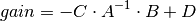
Returns:

gain: matrix

The gain of each output versus each input: $y = gain \cdot u$

Notes

This function is only useful for systems with invertible system matrix A.

All systems are first converted to state space form. The function then computes:

$gain = - C \cdot A^{-1} \cdot B + D$

control.matlab.drss(states=1, outputs=1, inputs=1)¶

Create a stable discrete random state space object.

Parameters:

states: integer

Number of state variables

inputs: integer

Number of system inputs

outputs: integer

Number of system outputs

Returns:

sys: StateSpace

The randomly created linear system

Raises:

ValueError

if any input is not a positive integer

See also

rss

Notes

If the number of states, inputs, or outputs is not specified, then the missing numbers are assumed to be 1. The poles of the returned system will always have a magnitude less than 1.

control.matlab.evalfr(sys, x)¶

Evaluate the transfer function of an LTI system for a single complex number x.

To evaluate at a frequency, enter x = omega*j, where omega is the frequency in radians

Parameters:

sys: StateSpace or TransferFunction

Linear system

x: scalar

Complex number

Returns:

fresp: ndarray

See also

freqresp, bode

Notes

This function is a wrapper for StateSpace.evalfr and TransferFunction.evalfr.

Examples

>>> sys = ss("1. -2; 3. -4", "5.; 7", "6. 8", "9.")
>>> evalfr(sys, 1j)
array([[ 44.8-21.4j]])
>>> # This is the transfer function matrix evaluated at s = i.

Todo

Add example with MIMO system

control.matlab.frd(*args)¶

Construct a Frequency Response Data model, or convert a system

frd models store the (measured) frequency response of a system.

This function can be called in different ways:

frd(response, freqs): Create an frd model with the given response data, in the form of complex response vector, at matching frequency freqs [in rad/s]
frd(sys, freqs): Convert an LTI system into an frd model with data at frequencies freqs.

Parameters:

response: array_like, or list

complex vector with the system response

freq: array_lik or lis

vector with frequencies

sys: LTI (StateSpace or TransferFunction)

A linear system

Returns:

sys: FRD

New frequency response system

See also

ss, tf

control.matlab.freqresp(sys, omega)¶

Frequency response of an LTI system at multiple angular frequencies.

Parameters:

sys: StateSpace or TransferFunction

Linear system

omega: array_like

List of frequencies

Returns:

mag: ndarray

phase: ndarray

omega: list, tuple, or ndarray

See also

evalfr, bode

Notes

This function is a wrapper for StateSpace.freqresp and TransferFunction.freqresp. The output omega is a sorted version of the input omega.

Examples

>>> sys = ss("1. -2; 3. -4", "5.; 7", "6. 8", "9.")
>>> mag, phase, omega = freqresp(sys, [0.1, 1., 10.])
>>> mag
array([[[ 58.8576682 ,  49.64876635,  13.40825927]]])
>>> phase
array([[[-0.05408304, -0.44563154, -0.66837155]]])

Todo

Add example with MIMO system

#>>> sys = rss(3, 2, 2) #>>> mag, phase, omega = freqresp(sys, [0.1, 1., 10.]) #>>> mag[0, 1, :] #array([ 55.43747231, 42.47766549, 1.97225895]) #>>> phase[1, 0, :] #array([-0.12611087, -1.14294316, 2.5764547 ]) #>>> # This is the magnitude of the frequency response from the 2nd #>>> # input to the 1st output, and the phase (in radians) of the #>>> # frequency response from the 1st input to the 2nd output, for #>>> # s = 0.1i, i, 10i.

control.matlab.impulse(sys, T=None, input=0, output=None)¶

Impulse response of a linear system

If the system has multiple inputs or outputs (MIMO), one input has to be selected for the simulation. Optionally, one output may be selected. If no selection is made for the output, all outputs are given. The parameters input and output do this. All other inputs are set to 0, all other outputs are ignored.

Parameters:

sys: StateSpace, TransferFunction

LTI system to simulate

T: array-like object, optional

Time vector (argument is autocomputed if not given)

input: int

Index of the input that will be used in this simulation.

output: int

Index of the output that will be used in this simulation.

Returns:

yout: array

Response of the system

T: array

Time values of the output

See also

lsim, step, initial

Examples

>>> yout, T = impulse(sys, T)

control.matlab.initial(sys, T=None, X0=0.0, input=None, output=None)¶

Initial condition response of a linear system

If the system has multiple outputs (?IMO), optionally, one output may be selected. If no selection is made for the output, all outputs are given.

Parameters:

sys: StateSpace, or TransferFunction

LTI system to simulate

T: array-like object, optional

Time vector (argument is autocomputed if not given)

X0: array-like object or number, optional

Initial condition (default = 0)

Numbers are converted to constant arrays with the correct shape.

input: int

This input is ignored, but present for compatibility with step and impulse.

output: int

If given, index of the output that is returned by this simulation.

Returns:

yout: array

Response of the system

T: array

Time values of the output

See also

lsim, step, impulse

Examples

>>> yout, T = initial(sys, T, X0)

control.matlab.lsim(sys, U=0.0, T=None, X0=0.0)¶

Simulate the output of a linear system.

As a convenience for parameters U, X0: Numbers (scalars) are converted to constant arrays with the correct shape. The correct shape is inferred from arguments sys and T.

Parameters:

sys: LTI (StateSpace, or TransferFunction)

LTI system to simulate

U: array-like or number, optional

Input array giving input at each time T (default = 0).

If U is None or 0, a special algorithm is used. This special algorithm is faster than the general algorithm, which is used otherwise.

T: array-like

Time steps at which the input is defined, numbers must be (strictly monotonic) increasing.

X0: array-like or number, optional

Initial condition (default = 0).

Returns:

yout: array

Response of the system.

T: array

Time values of the output.

xout: array

Time evolution of the state vector.

See also

step, initial, impulse

Examples

>>> yout, T, xout = lsim(sys, U, T, X0)

control.matlab.margin(*args)¶

Calculate gain and phase margins and associated crossover frequencies

Function margin takes either 1 or 3 parameters.

Parameters:

sys : StateSpace or TransferFunction

Linear SISO system

mag, phase, w : array_like

Input magnitude, phase (in deg.), and frequencies (rad/sec) from bode frequency response data

Returns:

gm, pm, Wcg, Wcp : float

Gain margin gm, phase margin pm (in deg), gain crossover frequency (corresponding to phase margin) and phase crossover frequency (corresponding to gain margin), in rad/sec of SISO open-loop. If more than one crossover frequency is detected, returns the lowest corresponding margin.

Examples

>>> sys = tf(1, [1, 2, 1, 0])
>>> gm, pm, Wcg, Wcp = margin(sys)

control.matlab.ngrid()¶

Nichols chart grid

Plots a Nichols chart grid on the current axis, or creates a new chart if no plot already exists.

Parameters:

cl_mags : array-like (dB), optional

Array of closed-loop magnitudes defining the iso-gain lines on a custom Nichols chart.

cl_phases : array-like (degrees), optional

Array of closed-loop phases defining the iso-phase lines on a custom Nichols chart. Must be in the range -360 < cl_phases < 0

Returns:

None

control.matlab.pole(sys)¶

Compute system poles.

Parameters:

sys: StateSpace or TransferFunction

Linear system

Returns:

poles: ndarray

Array that contains the system’s poles.

Raises:

NotImplementedError

when called on a TransferFunction object

See also

zero

Notes

This function is a wrapper for StateSpace.pole and TransferFunction.pole.

control.matlab.rlocus(sys, klist=None, **keywords)¶

Root locus plot

The root-locus plot has a callback function that prints pole location, gain and damping to the Python consol on mouseclicks on the root-locus graph.

Parameters:

sys: StateSpace or TransferFunction

Linear system

klist: iterable, optional

optional list of gains

xlim : control of x-axis range, normally with tuple, for

other options, see matplotlib.axes

ylim : control of y-axis range

Plot : boolean (default = True)

If True, plot magnitude and phase

PrintGain: boolean (default = True)

If True, report mouse clicks when close to the root-locus branches, calculate gain, damping and print

Returns:

rlist:

list of roots for each gain

klist:

list of gains used to compute roots

control.matlab.rss(states=1, outputs=1, inputs=1)¶

Create a stable continuous random state space object.

Parameters:

states: integer

Number of state variables

inputs: integer

Number of system inputs

outputs: integer

Number of system outputs

Returns:

sys: StateSpace

The randomly created linear system

Raises:

ValueError

if any input is not a positive integer

See also

drss

Notes

If the number of states, inputs, or outputs is not specified, then the missing numbers are assumed to be 1. The poles of the returned system will always have a negative real part.

control.matlab.ss(*args)¶

Create a state space system.

The function accepts either 1, 4 or 5 parameters:

ss(sys)

Convert a linear system into space system form. Always creates a new system, even if sys is already a StateSpace object.

ss(A, B, C, D)

Create a state space system from the matrices of its state and output equations:

$\dot x = A \cdot x + B \cdot u y = C \cdot x + D \cdot u$

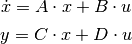
ss(A, B, C, D, dt)

Create a discrete-time state space system from the matrices of its state and output equations:

$x[k+1] = A \cdot x[k] + B \cdot u[k] y[k] = C \cdot x[k] + D \cdot u[ki]$

The matrices can be given as array like data types or strings. Everything that the constructor of numpy.matrix accepts is permissible here too.

Parameters:

sys: StateSpace or TransferFunction

A linear system

A: array_like or string

System matrix

B: array_like or string

Control matrix

C: array_like or string

Output matrix

D: array_like or string

Feed forward matrix

dt: If present, specifies the sampling period and a discrete time

system is created

Returns:

out: StateSpace

The new linear system

Raises:

ValueError

if matrix sizes are not self-consistent

See also

tf, ss2tf, tf2ss

Examples

>>> # Create a StateSpace object from four "matrices".
>>> sys1 = ss("1. -2; 3. -4", "5.; 7", "6. 8", "9.")

>>> # Convert a TransferFunction to a StateSpace object.
>>> sys_tf = tf([2.], [1., 3])
>>> sys2 = ss(sys_tf)

control.matlab.ss2tf(*args)¶

Transform a state space system to a transfer function.

The function accepts either 1 or 4 parameters:

ss2tf(sys)

Convert a linear system into space system form. Always creates a new system, even if sys is already a StateSpace object.

ss2tf(A, B, C, D)

Create a state space system from the matrices of its state and output equations.

For details see: ss()

Parameters:

sys: StateSpace

A linear system

A: array_like or string

System matrix

B: array_like or string

Control matrix

C: array_like or string

Output matrix

D: array_like or string

Feedthrough matrix

Returns:

out: TransferFunction

New linear system in transfer function form

Raises:

ValueError

if matrix sizes are not self-consistent, or if an invalid number of arguments is passed in

TypeError

if sys is not a StateSpace object

See also

tf, ss, tf2ss

Examples

>>> A = [[1., -2], [3, -4]]
>>> B = [[5.], [7]]
>>> C = [[6., 8]]
>>> D = [[9.]]
>>> sys1 = ss2tf(A, B, C, D)

>>> sys_ss = ss(A, B, C, D)
>>> sys2 = ss2tf(sys_ss)

control.matlab.ssdata(sys)¶

Return state space data objects for a system

Parameters:

sys: LTI (StateSpace, or TransferFunction)

LTI system whose data will be returned

Returns:

(A, B, C, D): list of matrices

State space data for the system

control.matlab.step(sys, T=None, X0=0.0, input=0, output=None)¶

Step response of a linear system

If the system has multiple inputs or outputs (MIMO), one input has to be selected for the simulation. Optionally, one output may be selected. If no selection is made for the output, all outputs are given. The parameters input and output do this. All other inputs are set to 0, all other outputs are ignored.

Parameters:

sys: StateSpace, or TransferFunction

LTI system to simulate

T: array-like object, optional

Time vector (argument is autocomputed if not given)

X0: array-like or number, optional

Initial condition (default = 0)

Numbers are converted to constant arrays with the correct shape.

input: int

Index of the input that will be used in this simulation.

output: int

If given, index of the output that is returned by this simulation.

Returns:

yout: array

Response of the system

T: array

Time values of the output

See also

lsim, initial, impulse

Examples

>>> yout, T = step(sys, T, X0)

control.matlab.tf(*args)¶

Create a transfer function system. Can create MIMO systems.

The function accepts either 1 or 2 parameters:

tf(sys)

Convert a linear system into transfer function form. Always creates a new system, even if sys is already a TransferFunction object.

tf(num, den)

Create a transfer function system from its numerator and denominator polynomial coefficients.

If num and den are 1D array_like objects, the function creates a SISO system.

To create a MIMO system, num and den need to be 2D nested lists of array_like objects. (A 3 dimensional data structure in total.) (For details see note below.)

tf(num, den, dt)

Create a discrete time transfer function system; dt can either be a positive number indicating the sampling time or ‘True’ if no specific timebase is given.

Parameters:

sys: LTI (StateSpace or TransferFunction)

A linear system

num: array_like, or list of list of array_like

Polynomial coefficients of the numerator

den: array_like, or list of list of array_like

Polynomial coefficients of the denominator

Returns:

out: TransferFunction

The new linear system

Raises:

ValueError

if num and den have invalid or unequal dimensions

TypeError

if num or den are of incorrect type

See also

ss, ss2tf, tf2ss

Notes

num[i][j] contains the polynomial coefficients of the numerator for the transfer function from the (j+1)st input to the (i+1)st output. den[i][j] works the same way.

The list [2, 3, 4] denotes the polynomial $2s^2 + 3s + 4$ .

Examples

>>> # Create a MIMO transfer function object
>>> # The transfer function from the 2nd input to the 1st output is
>>> # (3s + 4) / (6s^2 + 5s + 4).
>>> num = [[[1., 2.], [3., 4.]], [[5., 6.], [7., 8.]]]
>>> den = [[[9., 8., 7.], [6., 5., 4.]], [[3., 2., 1.], [-1., -2., -3.]]]
>>> sys1 = tf(num, den)

>>> # Convert a StateSpace to a TransferFunction object.
>>> sys_ss = ss("1. -2; 3. -4", "5.; 7", "6. 8", "9.")
>>> sys2 = tf(sys1)

control.matlab.tf2ss(*args)¶

Transform a transfer function to a state space system.

The function accepts either 1 or 2 parameters:

tf2ss(sys)

Convert a linear system into transfer function form. Always creates a new system, even if sys is already a TransferFunction object.

tf2ss(num, den)

Create a transfer function system from its numerator and denominator polynomial coefficients.

For details see: tf()

Parameters:

sys: LTI (StateSpace or TransferFunction)

A linear system

num: array_like, or list of list of array_like

Polynomial coefficients of the numerator

den: array_like, or list of list of array_like

Polynomial coefficients of the denominator

Returns:

out: StateSpace

New linear system in state space form

Raises:

ValueError

if num and den have invalid or unequal dimensions, or if an invalid number of arguments is passed in

TypeError

if num or den are of incorrect type, or if sys is not a TransferFunction object

See also

ss, tf, ss2tf

Examples

>>> num = [[[1., 2.], [3., 4.]], [[5., 6.], [7., 8.]]]
>>> den = [[[9., 8., 7.], [6., 5., 4.]], [[3., 2., 1.], [-1., -2., -3.]]]
>>> sys1 = tf2ss(num, den)

>>> sys_tf = tf(num, den)
>>> sys2 = tf2ss(sys_tf)

control.matlab.tfdata(sys)¶

Return transfer function data objects for a system

Parameters:

sys: LTI (StateSpace, or TransferFunction)

LTI system whose data will be returned

Returns:

(num, den): numerator and denominator arrays

Transfer function coefficients (SISO only)

control.matlab.zero(sys)¶

Compute system zeros.

Parameters:

sys: StateSpace or TransferFunction

Linear system

Returns:

zeros: ndarray

Array that contains the system’s zeros.

Raises:

NotImplementedError

when called on a TransferFunction object or a MIMO StateSpace object

See also

pole

Notes

This function is a wrapper for StateSpace.zero and TransferFunction.zero.