| Start the Lab 1 | Problem Set | Math Alive |
Birth, Growth, Death and Chaos. Part 1.
You can answer by filling in the blank spaces. If there is not enough space attach other sheets.
Problem 1. Amoebae troubles
Suppose we have a container in which there is an amoeba which splits into two halves in one minute, each one immediately growing to the same size as the parent. In 77 minutes the multitude of amoebae completely fill their container. To the nearest minute, how much time was needed to fill half of the container?
Answer:
Problem 2. Comparing different growth models
In this exercise you will compare simple proportional, square root, quadratic and exponential growth by plotting graphs of P(n)-the "population" at "time" n (for instance, after n years)- versus n. For these four cases you can compute the successive P(n) by the formulae given below:
| simple proportional: | P(n)=P(0)(1+rn) |
| square root: | P(n)=P(0)(1+rn)1/2 |
| quadratic: | P(n)=P(0)(1+rn)2 |
| exponential: | P(n)=P(0)(1+r)n |
To use these, you need to know what the initial population is, and you need to choose a value for r, a parameter that fixes growth rate in each case. For your graphs, pick P(0)=100; you get to pick your own value for "r", but you should keep it the same for all four cases. (It is a good idea to experiment a bit first with your choice of r: if you choose r really small, like 0.01, then you won't see much of a difference for n up to 10; if you choose r too large, like 2, then some of the growth curves may well grow so quickly that it is hard to make the comparison asked for below.)
Please compute P(n) for n=0,1,...,10 for each growth model (simple proportional, square root, quadratic and exponential) using the above formulae and fill up the following tables.
Answer:
Simple Proportional Growth:
| n | 0 | 1 | 2 | 3 | 4 | 5 | 6 | 7 | 8 | 9 | 10 |
| P(n) |
Square Root Growth:
| n | 0 | 1 | 2 | 3 | 4 | 5 | 6 | 7 | 8 | 9 | 10 |
| P(n) |
Quadratic Growth:
| n | 0 | 1 | 2 | 3 | 4 | 5 | 6 | 7 | 8 | 9 | 10 |
| P(n) |
Exponential Growth:
| n | 0 | 1 | 2 | 3 | 4 | 5 | 6 | 7 | 8 | 9 | 10 |
| P(n) |
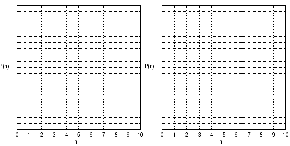
Now graph P(n) for n=0,1,...,10 for each case using the above tables on the Figures below.
 |
 |
Which one grows fastest initially?
Answer:
Which one wins in the end?
Answer:
How would P(n)=P(0)(1+rn)C compare with the others where C is some large CONSTANT positive number?
Answer:
Problem 3. Simple and Compound Interest
In the Online Lab, the first page of "Linear Models" reviews how one obtains the formulae for "simple proportional" growth (corresponding to a fixed interest rate without compounding) and "geometric" growth (corresponding to a fixed interest rate with compounding). Both these models are called "linear" because at any time step n, the population P(n) is just a multiple of P(0); the coefficient in the multiple varies with n, and also depends on which model you use, but it is independent of P(0) itself. An example: suppose that in one of these models with, say, a starting population of 1,000 you find that after 17 time steps it has increased to 9,720. Then, if you computed the population in the same model after the same number (17) of time steps, but starting from an initial population of 300,000 (300 times larger than before), you would find the result 2,916,000 (that is, 300 x 9,720). This will no longer be true for the family of models that you will study next under the heading "Non-linear growth".
In this exercise you will investigate properties of simple and compound interest. Use the graphing software provided in the second page of the Linear Models section in the Online Lab, whenever necessary. Suppose you have a certain amount of money, say $1000. In all cases we consider an annual interest rate of 3%, meaning that if we started with $1000, and took out the interest earnings whenever they are paid out, we would end up with $30 of total interest at the end of the year. We want to see the effect of compunding, i.e. of leaving all the interest income in the account so that it, in turn, can earn interest.
How much money would you have at the end of 5 years with an annual interest rate of 3% if the interest is compounded
—annually?
Answer:
—quarterly?
Answer:
—monthly?
Answer:
—every hour? (assume that the year
consists of exactly 365 days and
6 hours.)
Answer:
—every minute?
Answer:
You should observe that as you compound more and more often, the outcome changes less each time. If we compounded every second, or every 1/10 of a second, the outcome would be "almost" the same, i.e. as the compounding period approaches zero, the outcome tends to a certain number. This is what mathematicians call a "limit".
Using the graphing software provided in the second page of Linear Models section in the Online Lab, determine how many years later you will have at least the double amount of money with an annual interest rate of 10% assuming that the interest is compounded yearly? How long would it take to double your money if the interest was not compounded?
Answer:
Does your answer to the previous question depend on the initial amount of money you had? Justify your answer.
Answer:
Assuming that the interest is compounded annually, what would the interest rate have to be to double the amount of money?
—after 24 years?
Answer:
—after 12 years?
Answer:
Problem 4. Lottery
The New Jersey Lottery presents two options to the jackpot winners. Suppose you win a jackpot of $11 million. You can choose to get the money over 30 years with equal annual payments of $366,667, or you can choose to get the Lump-Sum cash value of $4.6 million, i.e. you receive $4.6 million in one payment immediately.
Suppose you decided to get the Lump-Sum cash value (of $4.6 million) and you use the total amount to buy a 30 year bond (meaning that you cannot cash it before 30 years have passed) that pays an annual percentage rate of 5.5% (compounded yearly). How much money will you have after 30 years?
Answer:
Suppose you choose to receive annual payments of $366,667 for 30 years; as soon as you receive your money every year, you invest it with a 5% annual interest rate (compounded yearly). How much will you have after 30 years?
Answer:
Which was the wise decision in this case?
Answer:
Would your answer have changed if you could have obtained a 5.5% interest rate every year for your annual investements of $366,667?
Answer:
The next section in the lab is on "Nonlinear Models". It reviews the formula for the logistic model. The second page introduces you to a graphical package with which you can explore the logistic model for this assignment. The way it works is very similar to the graphs you explored for linear growth models, except that you will now see TWO graphs inside the window. The lower graph shows how each Pn+1 is obtained from the previous Pn, by iterating (following the staircase) on the reproduction curve. At the same time, as these iterations proceed, a plot of population versus time appears as the upper graph.
Problem 5. Non-linear growth models
Let P0 =0.3 and on the figure below, calculate P1, P2, P3, P4 by hand.
Answer:
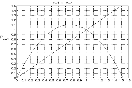
Do the same using the "spiral" or "staircase method" on the graph
below.
Answer:

Explain why this method works.
Answer:
Problem 6. Fixed points
In the Online Lab, there is a graphing software on the "Plotting Non-Linear Models" page. Set the initial condition P0 to 1, and plot the graph for N=20 for both r=1.9 and r=2.2. What do you observe? Can you explain why this point is called a "fixed point"?
Answer:
Now change the value of r to 1.9, and set P0 to some value very close to 1 (e.g. 0.95). Plot the curve again with N=50 using the software. What do you observe? Is the fixed point "stable" or "unstable" in this case?
Answer:
Do the same with r=2.2 this time. What do you observe? Is the fixed point "stable" or "unstable" in this case?
Answer:
Problem 7. Periodic behaviour
Using the graphing software in the
Online Lab, fill in the following table for r=2.1,
c=1
and
P0 =0.71 (round the numbers to three decimal
places)
Answer:
| n | 0 | 1 | 2 | 3 | 4 | 5 | 6 | 7 | 8 | 9 | 10 |
| P(n) | 0.71 |
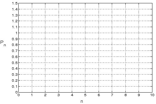
Now plot Pn versus n on the
graph paper provided below. What do you observe?
Answer:
Using the same values of r, c, and P0, calculate P200, P202 and P204. You should observe that they are equal to each other. Now calculate P201, P203 and P205. What do you see? In this case, we say that Pn is periodic with period 2. Without using the software, can you guess the value of P2000002? What about P67181921?
Answer:
Now change r to 2.5, and fill the following table (round the numbers to four decimal places).
Answer:
| n | 200 | 201 | 202 | 203 | 204 | 205 | 206 | 207 | 208 | 209 | 210 |
| P(n) | 0.7012 |
Is P(n) periodic again? If yes, what is the period?
Answer:
Now try r=2.5442. What is the period now? (Hint: First choose N large (for example, N=10,000) to allow the transients to go away. ("Transients" are the decaying oscillations that you saw in the Lab with r=1.9, starting from P(0) = 0.95, for example, before the dynamics settled down at the fixed point equal to 1). Then use the final value of your previous long run (in the box Pc) as the starting value of a shorter run, with N=100 for example. This will allow you to see the dynamics (top plot), and to determine whether or not it is periodic (i.e., repeats after 2, 4, ... iterations). Once you have a sense for what the period is by looking at the plot, you can verify your guess by starting again from the value obtained after the previous run, do a stepwise interation and make sure that you return to your starting value (to within 8 decimal places is adequate) after the right number of iterations (i.e., what you thought the period was). If not, your graphical guess for the period from the plot was too coarse. The period must be higher, or the behavior may not be periodic!)
Answer:
Challenge Questions
Problem C1. More on the Lottery
In Problem 4, you have compared the two options that NJ Lottery presents to Jackpot winners, and decided whether it is wiser to get the Lump-sum cash value, or the 30 equal annual payments, given the interest rates. However, in your calculations you assumed that you do not touch any of this money during the course of 30 years. To be more realistic, we will now assume that you will pay yourself a salary of 50,000 a year from this Jackpot money. We have the same options as before, that is you win a jackpot of $11 million. You can choose to get the money over 30 years with equal annual payments of $366,667, or you can choose to get the Lump-Sum cash value of $4.6 million, i.e. you receive $4.6 million in one payment immediately. If you choose to receive the annual payments of $366,667, you deposit $50,000 out of it in a checking account which pays 0% interest, and the rest you invest with a 5% annual interest rate (compounded yearly). Assuming that you spend all of the $50,000 you put into the checking account by the end of the year every year, how much will you have after 30 years?
Now, let's see what happens if you choose the other option. Suppose you decided to get the Lump-Sum cash value (of $4.6 million) . You take $50,000 every year, and you invest the rest with the same annual interest rate of 5%. Again assuming that you spend all of the $50,000 by the end of every year, calculate how much you will have at the end of 30 years. What was the wise decision?
Repeat the previous question but suppose now that the yearly inflation rate is 2%. Hint: A yearly inflation rate of r% means that the prices (of goods and services) will increase r% every year. That means to you have to increase your $50,000 spending by 2% each year.
Answer:
Problem C2. Loans & Mortgages
Suppose you get a $20,000 loan, which you will pay over 48 months (equal amounts every month for 48 months). What will be the monthly payments if the APR of your loan is 7%?
Again suppose you get a $20,000 loan, and your bank told you that you will be paying $700 a month for 36 months at the end of which the loan will be paid off. What is the annual percentage rate in this case?
Answer:
Problem C3. Bifurcation Diagram
We have seen in class that for 0 < r < 2, the fixed point for the logistic map is stable. At r = 2, we have a bifurcation: the fixed point is not stable anymore for r > 2; instead we have stable period-2 orbit. Figure 12 in lecture notes illustartes that there are other critical values of r, at which we have new bifurcations: at r = r4, the period-2 orbit becomes unstable, we have a stable period-4 orbit for r > r4 (but a period-2 orbit for 2 < r < r4). Similarly, we have again a bifurcation at r = r8, at which the period-4 orbit becomes unstable and we have a stable period-8 orbit for r > r8. Similarly, at r16, the period-8 orbit becomes unstable, and we have a stable period-16 orbit for r > r16.
Using the software on the "Plotting Non-Linear Models" page of the Online Lab, determine r4, r8 and r16.
Are the orbits periodic for all values of r? If not, try to find a value of r where you suspect there may no longer be periodic behavior, attach graphs, and explain.
Answer:
| Start the Lab 1 | Last Modified: August 2008 |